Paris-based Voxline Audio company has started in 2017 developing audiophile, hand-crafted loudspeakers and designing its associated electronics (Digital Adio Converter, Amplifying chain). Building on a collaboration with Ecole Polytechnique, ENSAM and Voxline, we led a 5-month characterizing study of these loudspeakers with IRCAM, focusing on :

• The acoustic emission directivity behaviour, measuring it by traditional means in achenoic environment
• A modelling of the transduction chain with extended Thiele-Small parameters (that is, classical Thiele-Small modelling with addition of nonlinear laws) in the Port-Hamiltonian System formulation for passive, energy-conserving components. This model was built with the final aim of:
  • Identifying the Thiele-Small (linearized behaviour) parameters to compare the loudspeaker to industry standards
  • Understanding the most influent sources of nonlinear behaviour, to exhibit controls on the harmonic distortion rate
  • Building a digital twin of the loudspeaker suitable for realistic simulations, enabling Voxline to try out different parameter values and have an insight of the output frequency response without having to hand-build another prototype
• The harmonic content of the response, studying it with both traditional spectrum analysis tools and recent methods such as Homophase Signal Decomposition [1]

A full report in French is available at the following link

1- Louspeaker description

The so-called "Vertex" loudspeaker features :

• a frame composed of polyurethane violon-bridge-like structures, aluminium-neoprene joints and birch fine panels
• membranes which are composites of kozo paper and linen sheet, impregnated with vinyl glue and eventually coated with graphite-based paint and polishes typically used in musical insturment crafting
• a motor combining a long, flat double coiled encased in a light composite blade, and a double magnets line generating the desired magnet field

The geometry of the loudspeaker is described in fig.1 and fig.2 and a few introductory remarks can be made on (i) the solidarity between the front and rear membrane, leading us to expect a dipolar behaviour - (ii) the overall linear shape of the loudspeaker, quite unusual, which motivated us to commit a modal analysis of the global structure - (iii) the absence of enclosure.

fig.1 : (left-top) Vertex loudspeaker description (bottom-right) Vertex and associated subwoofer representation

fig.2 : Vertex loudspeaker motor [View from top]

Note: New developments have led to a prototype featuring two separate motors for the two membranes, enabling control of the phase difference of the poles and in that way shaping the acoustical emission directivity.

2- Emission directivity behaviour

We measured the directivity behaviour of the Vertex loudspeaker in IRCAM achenoic chamber, using 20Hz-20kHz exponential chirps. The results observed on fig.3 are extremely close to those of a theoretical acoustical dipole, which confirms the dipolar behaviour. The company embraced this behaviour it as a way to promote use of its loudspeakers in omnidirectional environments (the figure, although not shown here, is absolutely symmetrical), such as a central installation in art exhibitions for example. This has been tested in October 2020 at the Bettencourt Awards Exhibition in Palays de Tokyo (consult the Awards scheme ).

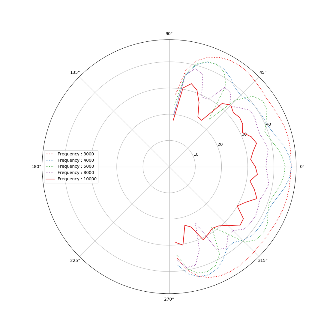
fig.3 : Vertex acoustical directivity diagrams [measured in achenoic environment with an exponential ascending chirp on a 20-20000Hz range] (left) Low-Frequencies (b) Mid-Frequencies (c) High-Frequencies

3- Physical modelling of the loudspeaker

We proposed 2 models for the loudspeaker : one being the classical, linear model involving Thiele-Small parameters and the other offering an extension of this linear model to take into account a nonlinear stiffness law and a nonlinear electromagnetic coupling function.

Linear model and Thiele-Small parameters

The most classical model derived by Thiele and Small in the mid 20th century features the following components and associated parameters :

• a coil with linear resistance $R_e$ and linear self-inductance $L_e$
• a pole-piece with electromagnetical coupling factor $B l $
• a suspension with damping factor $ R_{ms} $ and compliance factor $ C_{ms} $
• a membrane with mass $ M_{ms} $

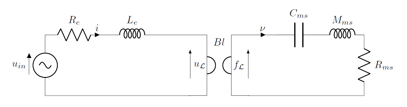
fig.4 : Linear model electromechanical equivalent circuit

This model greatly simplifies the physics at work by considering the Laplace force law does not depend on the geometry of the efficient field (which makes it linear with respect to the current by a coefficient $B l$ ). Also it suggests the stiffness law of the suspension is purely linear Hook, with stiffness $K_{ms} = \displaystyle{\frac{1}{C_{ms}}}$. Another impacting hypothesis is that the coil impendance is considered to be a linear inductance whereas numerous studies have shown the law is more sophisticated and [3][4] have proposed several models. Lastly it neglects loads of interactions and couplings within and between the electromagnetic and mechanical components (Eddy currents, Creep effect, Magnetic saturation in the pole piece...). We tried and took into account a few of these phonemena to take produce the next model ("extended" Thiele-Small).

Nonlinear model and extended Thiele-Small parameters

Studies like [5] have investigated the greatest sources of nonlinearities in loudpseaker physics and it results that the influence of membrane (equivalently coil) displacement over the electromagnetic coupling factor $B l$ was highly nonlinear, and that the stiffness law was far from linear Hook. We took these phenomena into account and came up with a similar model, where we added nonlinear laws for stiffness and electromagnetic coupling in the form of series in powers of displacement : \begin{align*} Bl(q) & \quad = \displaystyle{\sum_{n=0}^{N_B}} Bl_n q^n\\ K_{ms}(q) & \quad = \displaystyle{\frac{1}{C_{ms}(q)}} = \displaystyle{\sum_{n=1}^{N_K}} K_n q^n \end{align*} The objective of putting the nonlinear law in that form is that it provides us with polynomial laws easy to derive and include in a State-space/Volterra formalism. Indeed, as we will present it in the following section , we use that formalism to exploit the recurrent identification scheme proposed by [1]. Taking the outputs as the vector of membrane displacement $q$ and coil current intensity $i$, the input being the coil voltage $u_{in}$, we obtain the following State-space-representation equations : \begin{equation} \text{State} \ : x(t) = [ \phi(t), q(t), M_{ms} \frac{dq}{dt}(t) ]^T , \quad \text{Output} \ : y(t) = [ i(t), q(t)]^T , \quad \text{Input} \ : u(t) = u_{in}(t) \end{equation} \begin{align*} \text{Dynamic law} : & \quad \partial_t x(t) = Ax(t) + Bu(t) + \displaystyle{\sum_{n=2}^{N_B}} \mathcal{B}_n(x(t)) + \displaystyle{\sum_{n=2}^{N_K}} \mathcal{K}_n(x(t))\\ \text{Input-Output Law } : & \quad y(t) = C x(t) + D u(t) \\ \end{align*} \begin{align*} A & \quad = \begin{bmatrix} -\frac{R_e}{L_e} & 0 & - \frac{Bl_0}{M_{ms}} \\ 0 & 0 & \frac{1}{M_{ms}} \\ \frac{Bl_0}{L_e} & -K_1 & - \frac{R_{ms}}{M_{ms}} \\ \end{bmatrix} & \quad B & \quad = \begin{bmatrix} 1 \\ 0 \\ 0 \\ \end{bmatrix} \\ C & \quad = \begin{bmatrix} \frac{1}{L_e} & 0 & 0 \\ 1 & 0 & 0\\ \end{bmatrix} & \quad D & \quad = \begin{bmatrix} 0 \\ 0 \\ \end{bmatrix} \\ \mathcal{B}_n (x(t)) & \quad = \begin{bmatrix} - Bl_{n-1} \frac{dq}{dt}(t) q^{n-1}(t) \\ 0 \\ Bl_{n-1} \phi(t) q^{n-1}(t) \\ \end{bmatrix} & \quad \mathcal{K}_n(x(t)) & \quad = \begin{bmatrix} 0 \\ 0 \\ -K_n q^n \\ \end{bmatrix} \end{align*}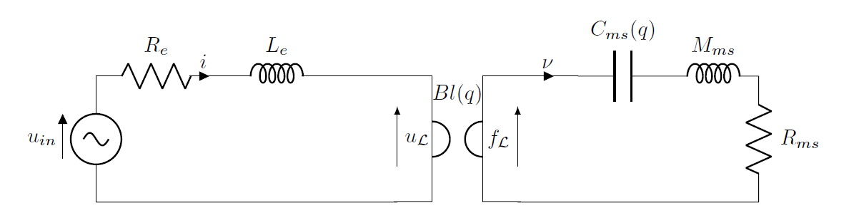

fig.5 : Nonlinear model electromechanical equivalent circuit

4- Identification of nonlinear parameters

Identification scheme

Our first assumption for using an identification scheme is that the modelled system is causal and representable with a Volterra Series formalism, that is, that we can link the input $u$ to the output $y$ with a Volterra operator $V$ defined as : \begin{equation} y(t) = V[u](t) = \displaystyle{ \sum_{ n \in \mathbb{N}^*} \int_{ \mathbb{R}_+^n} k_n(\tau_1, ..., \tau_n ) u(t - \tau_1)... u(t - \tau_n) d \underline{\tau}} \\ \end{equation} where $\{ k_n \}_{n \in \mathbb{N}}$ are the Volterra kernels of the system. These can be considered as an extension of the classical impulse reponse used in Liner-Time-Invariant systems (the kernel $k_1$ being that impulse response for the linearized system). The analogy is extendable to the Laplace domain, as we define the Volterra transfer kernels $H_n$ with: \begin{equation*} H_n(s_ 1, \dots, s_n) = \int_{ \mathbb{R}_+^n } h_n(\tau_1, \dots, \tau_n) e^{-( s_1 \tau + \dots + s_n \tau_n) } d\underline{\tau} \end{equation*} With these notations, the linearized system (i.e. the linear model presented in this subsection) is then characterized by the first transfer kernel $H_1(s) = \displaystyle{\frac{Y(s)}{U(s}}$. The link between this Volterra formalism and the State-space representation of a dynamic system is immediate for weakly nonlinear systems . These systems are defined by the following : if we mark the input by a scaling factor $\epsilon$ such as $u(t) = \epsilon v(t)$, then the output (and similarly for the state) can be derived as $y(t) = \displaystyle{\sum_{n \in \mathbb{N}}} \epsilon^n y_n$ where the $\{ y_n \}_n$ are called homogeneous orders . In that way, the system laws can be put in the following form : \begin{align*} \text{Dynamic law } : & \quad \partial_t x(t) = A x(t) + B x(t) + \displaystyle{\sum_{\substack{[p, q] \in \mathbb{N}^2 \\ 2 \leq p + q } }} \mathcal{M}_{p, q} \left( x, ....x, u, ..., u \right) (t)\\ \text{Input-Output law } : & \quad y(t) = C x(t) + D u(t) + \displaystyle{\sum_{\substack{[p, q] \in \mathbb{N}^2 \\ 2 \leq p + q } }} \mathcal{N}_{p, q} \left( x, ....x, u, ..., u \right) (t) \end{align*} with the $\mathcal{M_{p, q}}$ and $\mathcal{N_{p, q}}$ functions regrouping the nonlinearities of the system. Then, the link to the Volterra formalism is made by a computation formula of the transfer kernels called cancelling kernels method [2] (equation 2.26): \begin{equation} {\scriptstyle H_n(s_ 1, \dots, s_n) = W(\sum_{i=1}^n s_i) \Bigg( \displaystyle{ \sum_{ \substack{[p, q] \in \mathbb{N}^2 \\ 2 \leq p + q \leq n } }} \left[ \scriptstyle \mathbb{1}_{p \geq 1} %Cas p non-nul \displaystyle{ \sum_{ \substack{ m \in \left( \mathbb{N}^{*} \right)^p \\ m_1 + .. m_p = n - q} }} \scriptstyle \mathcal{M}_{p, q} \left( H_{m_1}(s_1, \dots, s_{m_1}), ....H_{m_p}(s_{m_1} + ... + s_{m_{p-1}+1}), 1, ..., 1 \right)\right] \scriptstyle + \mathcal{M}_{0, n} \left( 1, ..., 1 %Cas p = 0 \right) \Bigg) } \end{equation} The identification and validation process then consists in :

• Evaluating the homogeneous orders $(x_n, y_n)$ with a homogeneous separation scheme presented in [1] and explained in the report (section 2.3.4). This separation scheme uses experimental data measured on the loudspeaker with a special set of exciting signals, and collected with displacement and current sensors.
• Estimating the functions $\mathcal{M_{p, q}}$ and $\mathcal{N_{p, q}}$ and finally the nonlinear parameters through an iterative evaluation presented in [1] and explained in the report (section 3.5.1)
• Computing the transfer kernels with the above formula to get the Volterra representation of the system
• Resimulate with the estimated parameters and the corresponding transfer kernels the homomogeneous orders by mean of an orders realisation scheme described in [1]
• Compare the extracted homogeneous orders to their simulated counterparts and conclude on the validity of our nonlinear model

Identification results on Voxline Vertex prototypes

We used a PAS separation scheme ([1] and report , section 2.3.4) to extract and simulate 7 homoegeneous orders. The orders comparison is made in fig.6 , and we can make the following statements :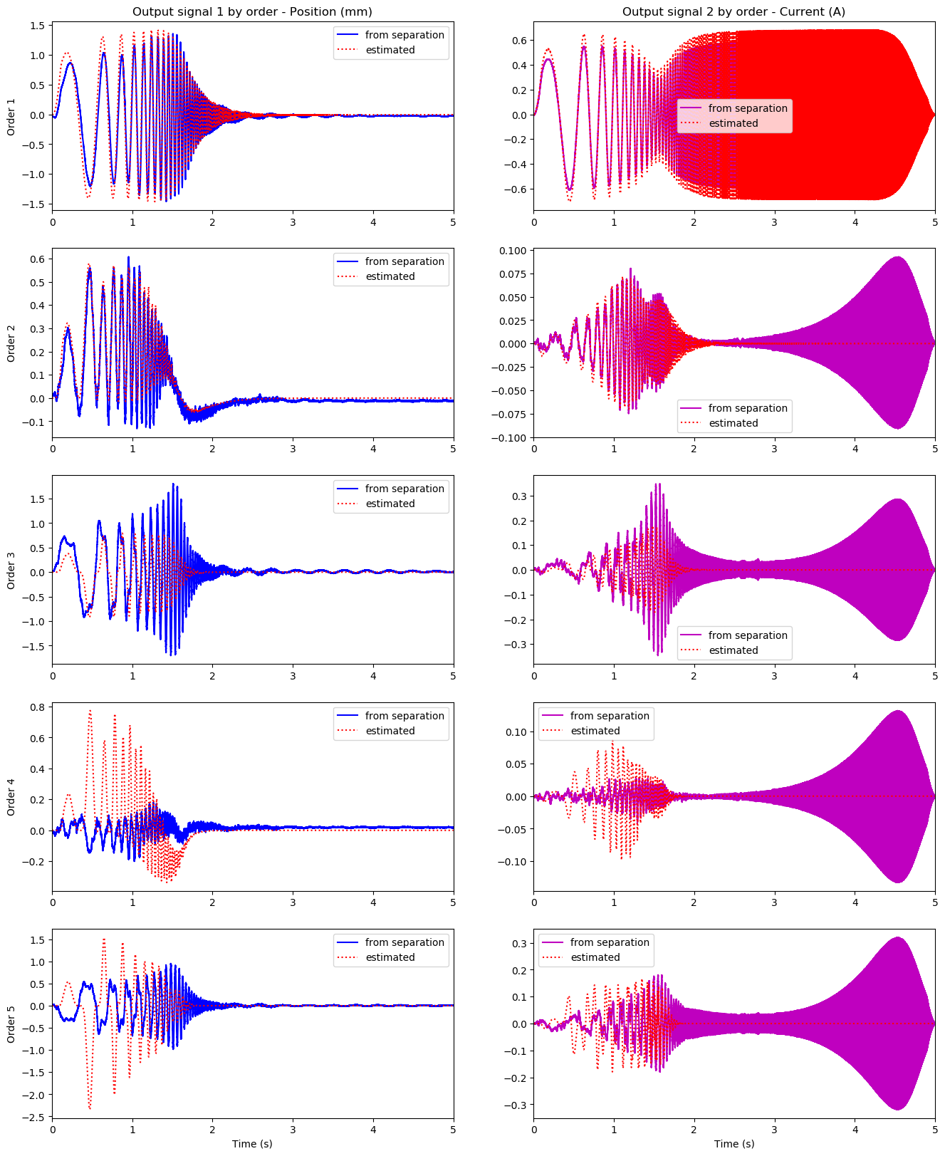

fig.6 : Homogeneous orders in membrane displacement (left) and coil intensity (right) in Vertex

• The separation scheme is dysfunctional for high frequencies, as we can notice digital oscillations in high frequency content on the intensity orders
• As we are forced for computation to truncate the Volterra series to a certain order $N$, estimation errors are introduced in the process given the lacking contributions from higher order transfer kernels. These errors have more impact on both the identification and realisation processes as the truncation order decreases.
• The estimation is better for low orders than for higher ones, since low orders get more contributions from transfer kernels in the orders realisation scheme. This leads us to chose a maximal order above which we will not use the extracted parameters for the estimation of the nonlinear laws.

When it comes to results, we can observe that the nonlinear orders have a large contribution to the total system response (the 3rd order response is almost similar in amplitude to the linearized system response (1st order)), which confirms our first intuition that such a geometry and choice of materials would introduce lots of nonlinearities. Also, the even-order contributions prove to be very high in this loudspeaker response, as the ratio of 2nd order to 1st order in the displacement response attains almost 40% (versus 2.5% in a classical Fostex loudspeaker that we used as a reference for our method: see fig.7 ). In general, odd orders are much more predominant because of the symmetry in the nonlinear laws, but in that particular case this even-order influence is relatable to the assymmetry in the shape and building of the membrane and suspension.

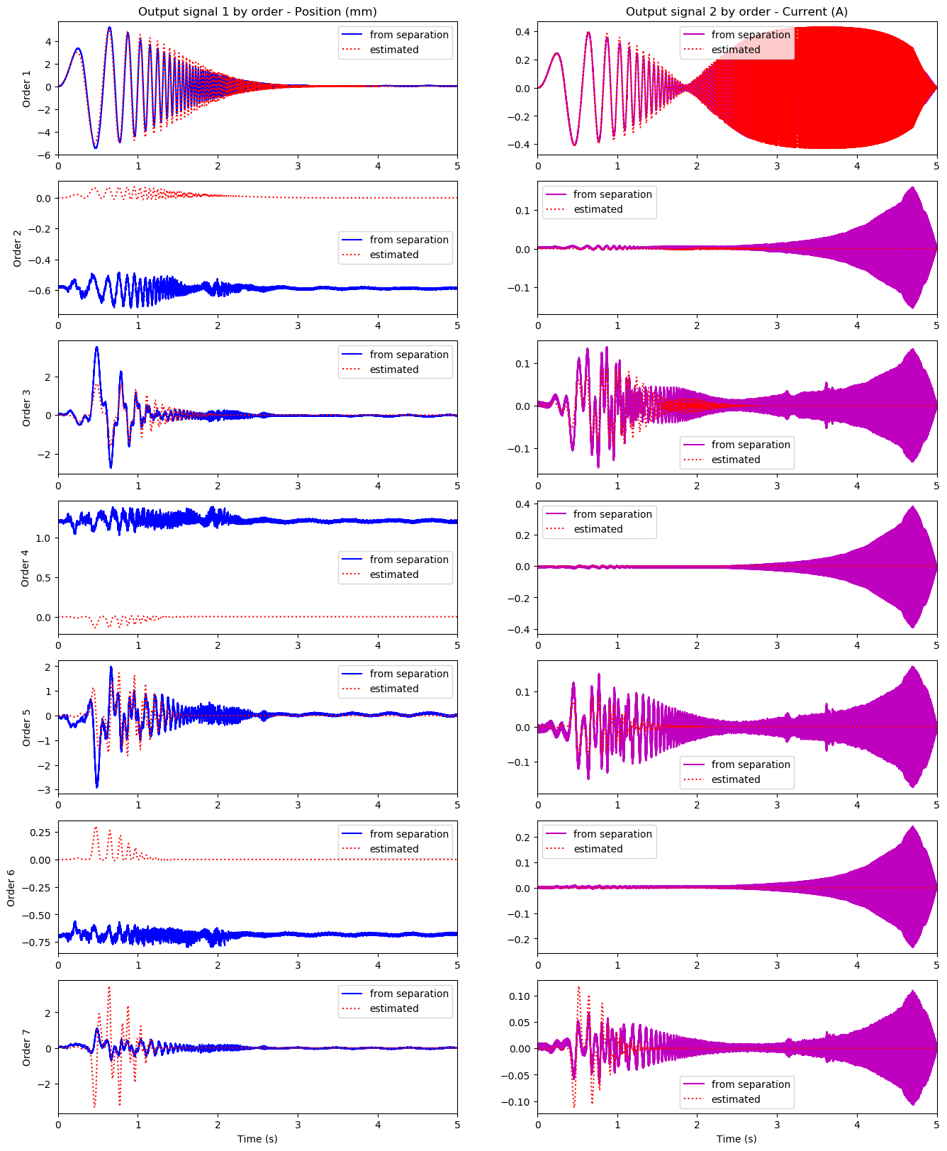
fig.7 : Homogeneous orders in membrane displacement (left) and coil intensity (right) in reference speaker (Fostex FE208ES). (Offsets in the odd-order response are an artifact unresolved yet).

We chose a truncation order of 3 (for the reasons given above) for the identified parameters to contribute to the electromagnetic coupling and stiffness laws: the results are displayed in fig.8, and suggest that the equilibrium point for the electromagnetic coupling (i.e. the point of maximal effective magnetic field) is shifted by about 1mm with respect to the center of the loudspeaker in that design. Also, with usual loudspeakers we observe a "hard-point" phenomenon, that is, a region close to the equilibrium point where the stiffness is higher than expected : we observe this for the reference loudspeaker (see fig.8 on right plot), but not for the Vertex loudspeaker (althoug the estimation seems quite rough since far from the equilibrium point, the stiffness seems to greatly decrease) .

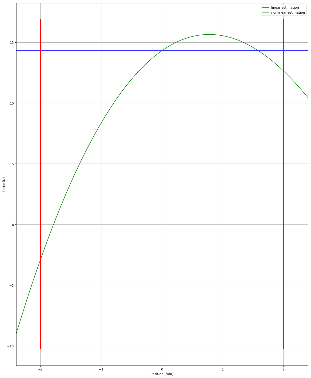
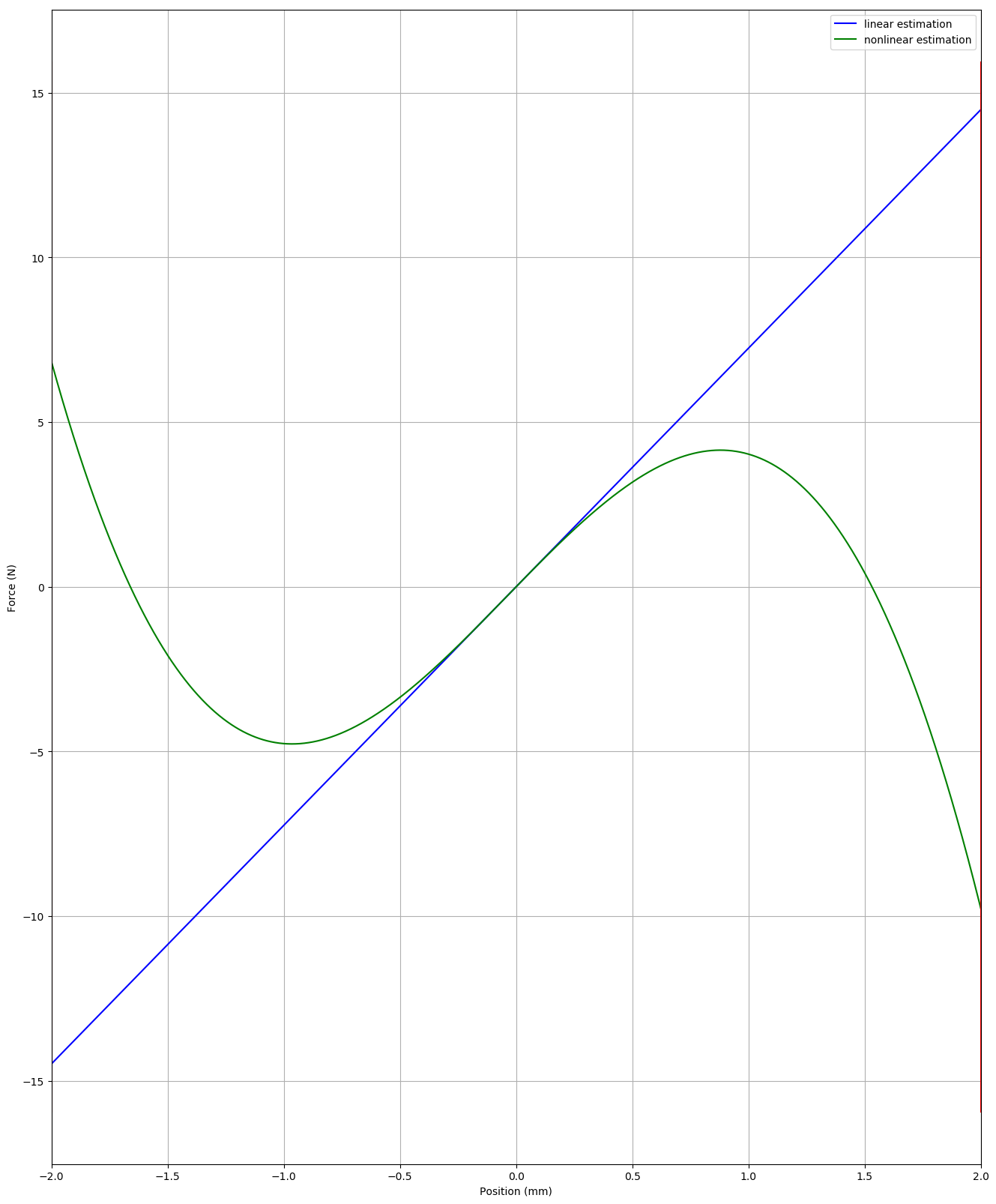
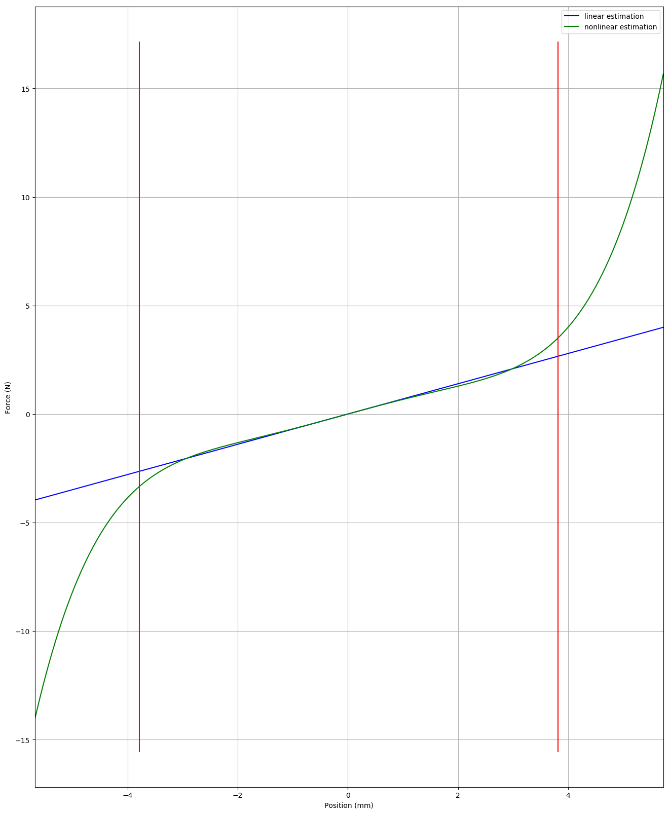
fig.8 : Electromagnetic coupling law (left) and Stiffness law (middle) for Vertex loudspeaker. Stiffness law (right) of reference loudspeaker

References

• [1] Damien Bouvier, Identification de systèmes non linéaires représentables en séries de Volterra: applications aux systèmes sonores, 2018
• [2] Thomas Helie,Modélisation physique d’instruments de musique et de la voix : Systèmes dynamiques, problèmes directs et inverses, 2013
• [3] Antoine Falaize, Thomas Helie. Passive modelling of the electrodynamic loudspeaker : from the Thiele-Small model to nonlinear Port- Hamiltonian Systems, 2018 hal-01874945.
• [4] Wolfgang Klippel. Sound Quality of Audio Systems, 2018. Course on Audio Systems, Technische Universität Dresden
• [5] Romain RAVAUD, Guy LEMARQUAND, Valérie LEMARQUAND, Tangi ROUSSEL Ranking of the Nonlinearities of Electrodynamic Loudspeakers, January 2010, Archives of Acoustics 35